Causal Intervention on a 2D Manifold of a Concept Family

In the previous post: ← Concept Geometry, we saw that concept families can be extracted and have real semantic structure in low dimensional sub-spaces. Days of the week condense to a circular structure with a break from "Sunday" to "Monday", with the radial extent increasing as the week proceeds. Months of the year are elliptical in earlier layers, where temporal structure lives, before fracturing off the 2D manifold into higher dimensional spaces. Compass directions similarly move from spatial directions in 2D to more correlational concepts in later layers.

I decided to look into this because I wanted to gain more intuitive understanding of multi-dimensional features. Chris Olah and Adam Jermyn outline Multi-dimensional features here: Chris Olah on Multidimensional Features.

In particular they state:

The more interesting requirement is Intensity as Scaling which significantly constrains the geometry of possible manifolds. Every point on the manifold forms a "ray" as you scale it, representing that feature at different levels of intensity. Jointly these form a path by which the entire manifold contracts back to zero. Then semantic changes need to be angular movement orthogonal to this.

There is lots in there, but I wanted to test one part of this — that angular position on the manifold encodes semantic identity within a concept family, and that this encoding is causally used by the model.

Reading from the Residual Stream

As shown previously, days of the week can be projected to a 2D manifold and show a relatively circular structure that was relatively robust with respect to transformer layer. This could be due to a few reasons (this is a non-exhaustive list): The days of the week are fairly unassuming concepts. There is not as much semantic loading in these tokens in training data generally. History might recall the year an event took place, potentially a time of the year, but it's unlikely the fine grained details trickle down to the day.

Suppose you ask your friend when the fire of London was, "1666" they say, looking pleased with themselves. "Great!" you respond, "what about the month?". They look at you a bit funny but your other friend pipes up—"September, I think the 2nd?". "Yes correct!" At this point your friends go back to discussing what they were discussing before you rudely interrupted..."What day was it?".

Silly anecdotes aside the point is that the fine grain detail of the days of the week do not have as much historic weight. Of course, there is "good friday" and "shrove tuesday", but when you compare against all the historical content that has a more well-known associated month of the year, it is intuitive to suppose the months start existing on a higher dimensional manifold.

A natural extension, therefore, is whether the model also reads from the day of the week manifold in a similar way. To test this, we develop a simple experiment to test whether making changes in the 2D manifold in early layers translates to quantitatively different outcome predictions.

Recall the PC space of a 2D manifold for the days of the week.

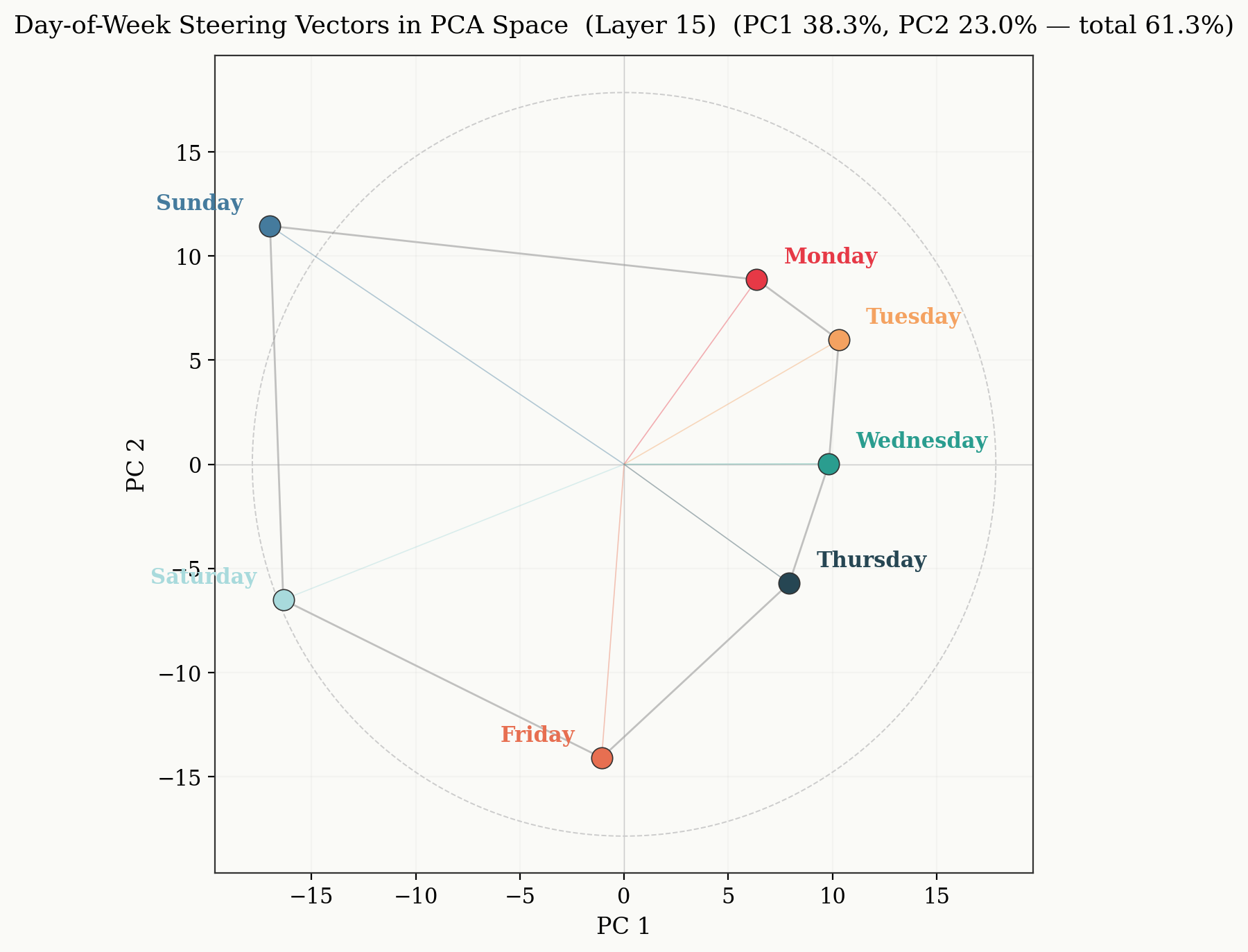
We start with the extracted vector of a given day of the week, and project into the 2D space (in this work, we started with the vector for "Monday"). Applying the learned rotation matrix, R, with different rotation angles (theta) we sweep out a unit circle centered on (0,0). At 10 degree increments we find the difference between the original steering vector and the steering vector we get by projecting the rotated vector back into the residual stream dimension.

Let P be the (2, D) matrix whose rows are the first two principal components. For a steering vector x in D-dimensional space, we rotate only its projection onto the 2D manifold:

x' = x + Pᵀ(R(θ) - I)Px

This applies rotation R(θ) to the 2D component while leaving the orthogonal complement unchanged. We sweep θ from 0° to 360° in 10° increments, inject x' as a steering vector—in this work, at layer 15—and record output probabilities.

We use a very simple prompt because the actual prompt nature is not that important, we want to see the empirical effects of injecting this vector relative to not injecting. Prompt = "What day does it feel like? Answer like this: day: "

We now find X' for rotations in PC space every 10 degrees, inject the vector, and record the output probabilities of each day of the week being selected to the prompt "What day does it feel like? Answer like this: day: ".

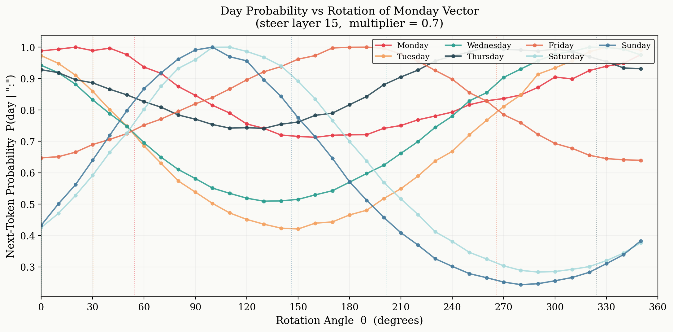
As the steering vector sweeps the 2D PC space, the probability for each day of the week being selected follows sinusoidal motion. This shows real causal intervention: by injecting a vector that is purely the difference in a rotation the 2D PC space, we see temporal effects in the predicted outcomes. Note, the probabilities of each day being predicted are normalised to their own maximum. This was a choice to show the sinusoidal result, at steering vector strengths of 0.7, the selected day only oscillated between "Wednesday" and "Friday".

As the injected vector strength increased, the sinusoidal pattern remained, however the width of the peak and trough of each day followed (identical) patterns of wider troughs and more narrow peaks. For increasing strengths this pattern continues with troughs becoming a wide flat minima and a singular peak. It seems that some days are never going to have the maximum probability, even when at the peak of their own probability curve. This might be internal bias in the model created during pre-training, or the particular choice of prompt. When seeing the effect of other prompt choices e.g. "What day does it not feel like", we see different days dominate the output probabilities. This is interesting in itself; the model has some prior over its favourability of each day, again likely due to the text seen during pre-training. Finally, for strengths greater than ~1.2, the regime breaks down and there is no obvious structure to discern.

Plotting the angular distance between consecutive day maximums as a function of the angle between consecutive days in PC space we get the following.

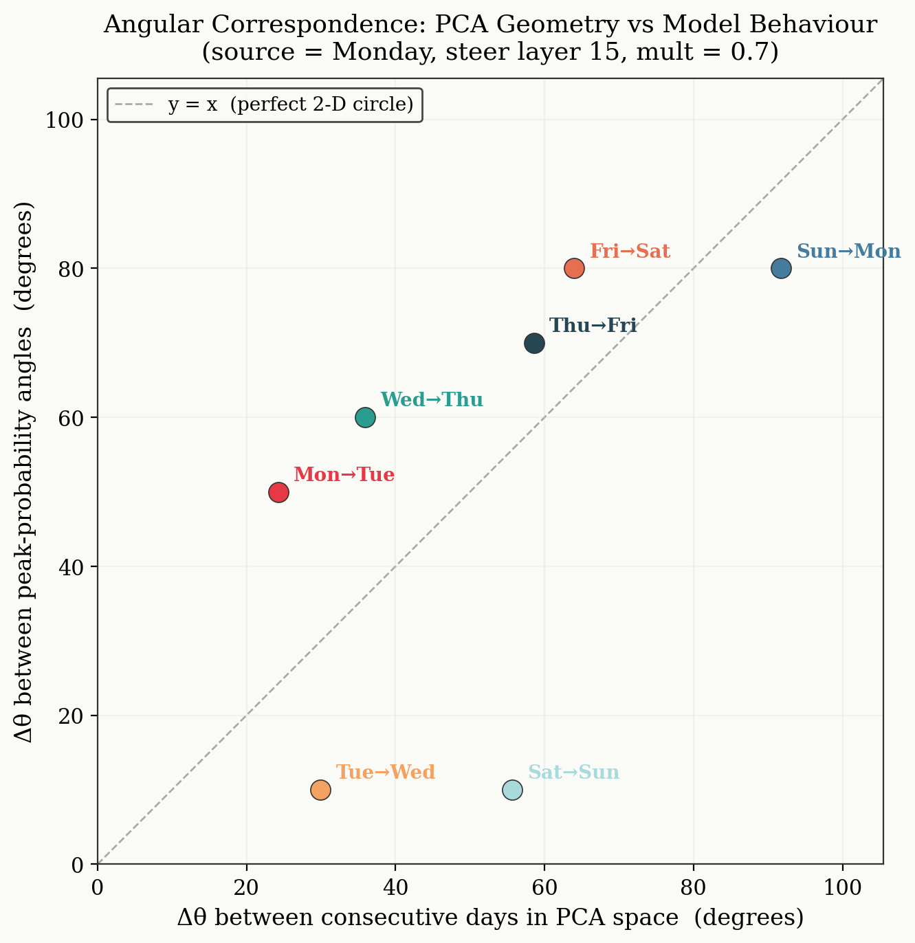
We might expect that if the model perfectly wrote to and read from a unit circle in 2D space, we would see the points lying on the y-x line, as rotations in the 2D manifold would perfectly correlate with maximum predicted probabilities. I am not making a claim that strong here, as I don't actually know if that is true. What we can claim, is that the fit is not dreadful, there is clustering near y=x for different consecutive day transitions. This fit isn't perfect for a few reasons. Firstly, the 2D manifold we use here encompasses about 60% of the total variation. Secondly, the days do not lie on a perfect circle, and the angular difference between consecutive days is not 360/7 ~ 52 degrees.

To me what is most outstanding is that the probabilities follow clean sinusoidal curves, and that rotating in this 2D subspace produces smooth, predictable changes in output probabilities. It is also important that the angular gaps between consecutive day peaks roughly correspond to the angular gaps in PCA space. The correspondence isn't perfect but it's there, and that's the real evidence that the model reads from this subspace.

Discussion

The findings here represent a causal result (not just observed geometry), and it works with only ~60% of variance captured. The sinusoidal structure suggests the model is performing roughly linear readout from the 2D subspace during the forward pass. These results are in line with what Chris describes for multidimensional features, with orthogonal movements corresponding to different semantics. We do not show in this work the causal impacts of changing the strengths of a given "ray", which we leave to future work.

Another obvious next step would be to try this method with months of the year (where the 2D manifold is less stable) to see if causal control breaks down in later layers where the geometry fractures.

All code and figures were produced using contrastive activation extraction on the Qwen3 13B parameter model, with thinking disabled. This model has separate Query heads for each of the 40 layers, however uses 8 Key and Value heads. The analysis requires only PCA, least-squares fitting, and SVD — no specialised interpretability tooling needed.

A Quick Aside

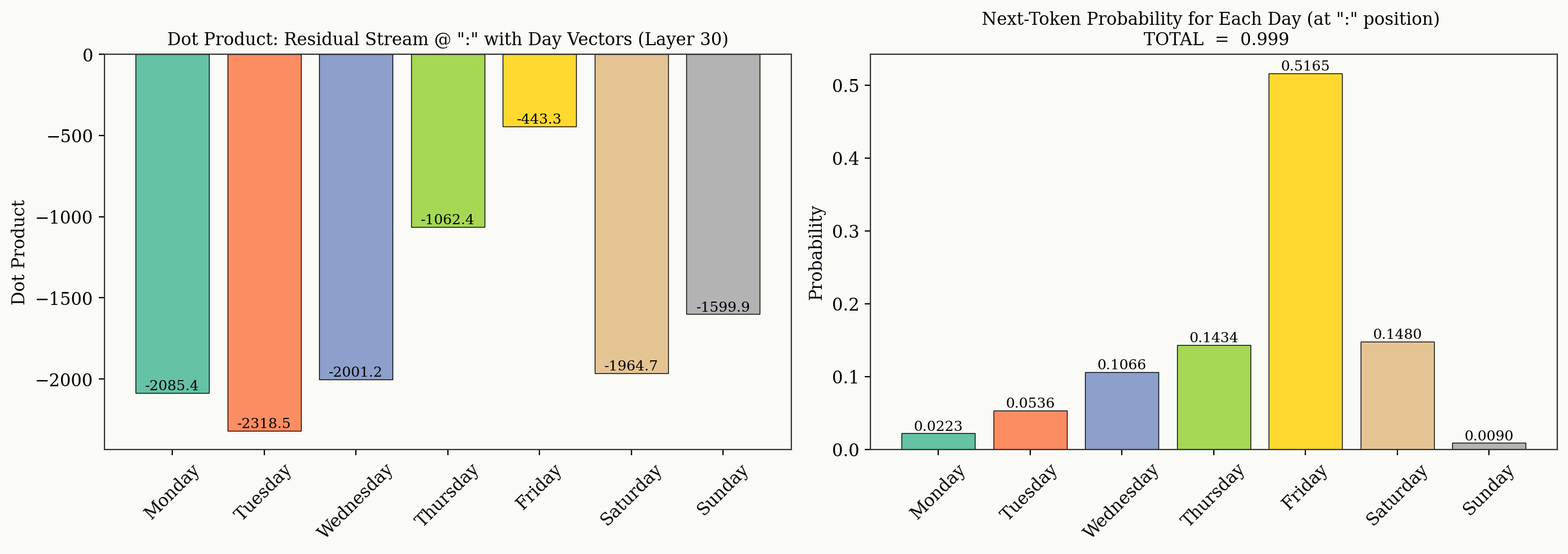
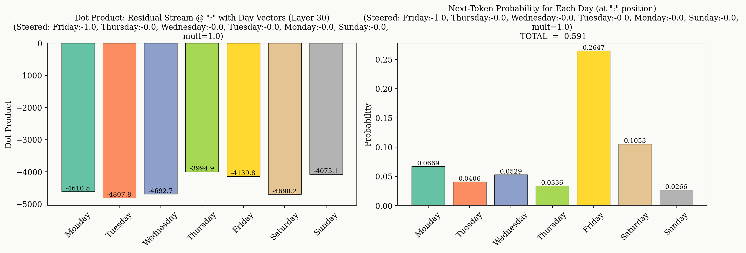
For completeness, we include a baseline analysis of the prompt used throughout this experiment we show the dot product between the individual day vectors and the residual stream at layer 30, alongside the output logit probabilities. In this case, "Friday" is the day it feels like, and we see the residual stream most closely aligns with "Friday". If we inject "Friday" with strength -1, we see all dot products drop—as expected, recall the days of the week all have high cosine similarity—however "Friday" remains the most likely day of the week, even though there is similar alignment between the residual stream and all other days of the week at layer 30. The model must be necessarily biased towards "Friday" (in this case) when deciding on an output prediction, this may be because the models prior is biased towards "Friday" for this prompt.

AI assistance

I use the pronoun "we" because this work was heavily influenced by AI. In particular, Opus 4.5 wrote ~75% of the code for this project, and ~100% of the plotting code.

I also used Opus 4.5 to discuss some of the key findings in this work, in order to cement my understanding and ensure my discussion was more structured.