The Geometry of Concept Families in Language Model Residual Streams

Steering vectors and concept vectors have become a popular tool in mechanistic interpretability — extract the direction in activation space that corresponds to a concept, and you can read off or even control the model's behaviour along that axis. But most work focuses on single concepts: truthfulness, sentiment, refusal. What happens when we look at families of related concepts together? Do the days of the week, the months of the year, or the compass directions form structured manifolds in the residual stream? And if so, what does the geometry tell us about how the model understands these concepts?

In this post, we extract steering vectors for several concept families from the Qwen3-13B model and show that they occupy low-dimensional subspaces with interpretable geometric structure. Days of the week form a spiral (consistently throughout the model layers). Months of the year form something closer to an ellipse (in certain layers). Compass directions form a clean square at some layers and a distorted trapezoid at others. The geometry does not seem arbitrary — it reflects both the true structure of the concept whilst showing signs of statistical patterns of language the models will have been trained on.

Extracting Concept Vectors

The approach is straightforward contrastive activation extraction (I use the steering-vector library: steering-vectors). For each concept in a family (e.g. "Monday", "Tuesday", ...), I get a LLM to generate ~20 prompt pairs where the positive prompt contains the concept and the negative prompt is a matched control without it. For example:

Positive: "The meeting is scheduled for Monday"
Negative: "The meeting is scheduled"

The steering vector for each concept is the mean difference in residual stream activations (at the last token position) between positive and negative prompts, computed at a specific layer(s). This gives us one high-dimensional vector per concept per layer. To visualise the relationships between concepts, we can project these vectors into a shared low-dimensional space using Principal Component Analysis (PCA - this finds the linear combination of vector components which maximise the variance along this linear projection between vectors in your set of vectors).

Days of the Week: A Spiral/Circle

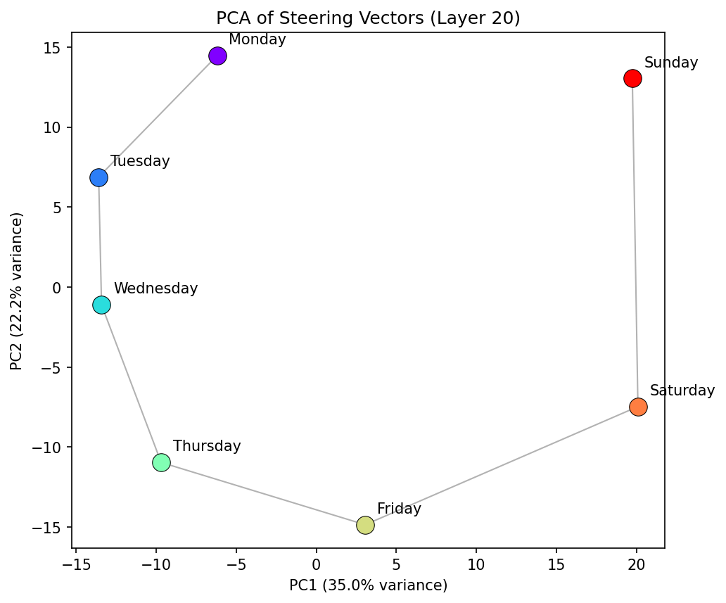
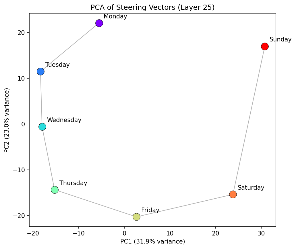
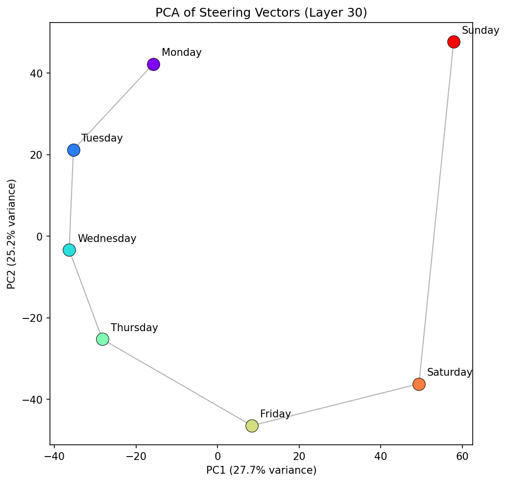
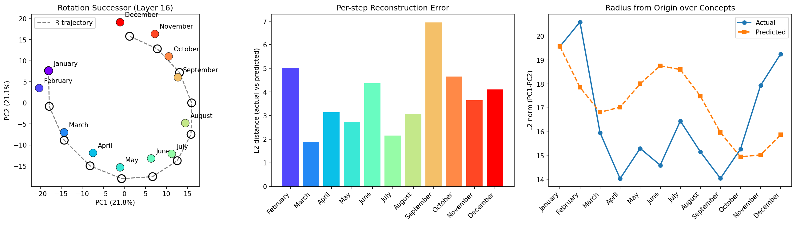
The first result is interesting, though not completely surprising: Projecting the seven day-of-week steering vectors into their first two principal components reveals an approximately circular arrangement — Monday through Sunday appear in clockwise order (in this instance; it can and does orient anti-clockwise too), with consecutive days as nearest neighbours. We see that the general PCA space representation is consistent over multiple middle to late layers, suggesting the manifold is inherently robust during a forward pass.

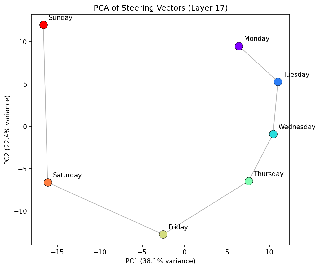
This is reiterated by showing how the cosine similarity between "Monday" and every other day varies as function of layer. From layer ~10 onwards there is a relatively constant structure, with all days following the same pattern.

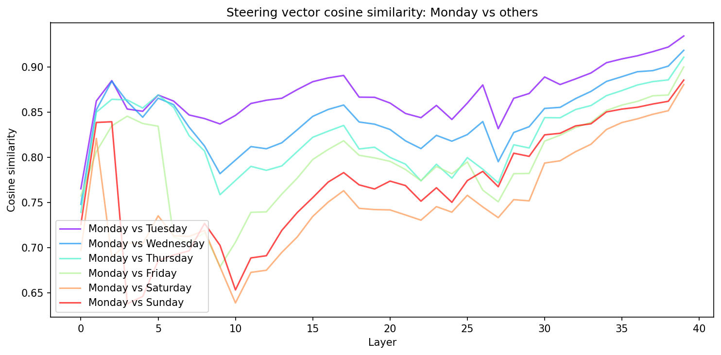
But, the PCA of this concept family is not quite a circle — it's more of a spiral in 2D. The radius increases from Monday through to Sunday, and there's a clear spatial gap between Sunday and Monday. The model has learned the sequential ordering of the week, but treats it more as a linear progression than a periodic cycle. Sunday and Monday are the most distant consecutive pair, suggesting the model represents a "week boundary" rather than a smooth wrap-around we might expect of a perfectly periodic concept family.

This is probably unsurprising from a training data perspective. In natural language, the week is often described linearly — "from Monday to Friday", "the weekend", "next week starts on Monday" — with an implicit break between Sunday and the following Monday. The geometry of the representation reflects the geometry of the language. "Monday" is still the next closest to "Sunday" after "Saturday" but the clean continuation is not there. This finding is pretty robust to different layers too as we see below.

Fitting a Rotation Matrix

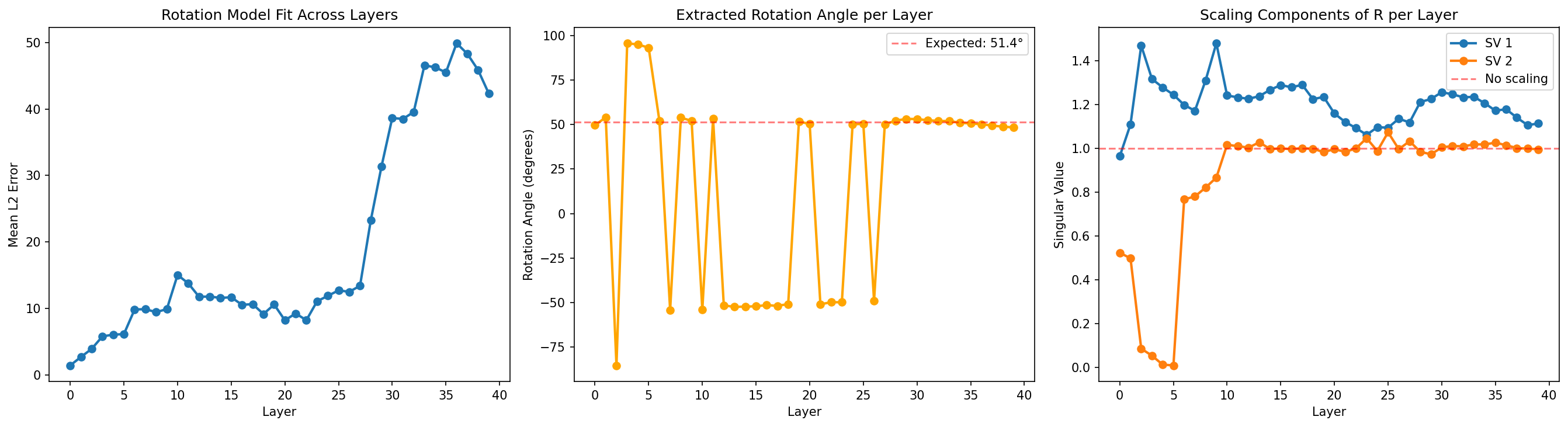
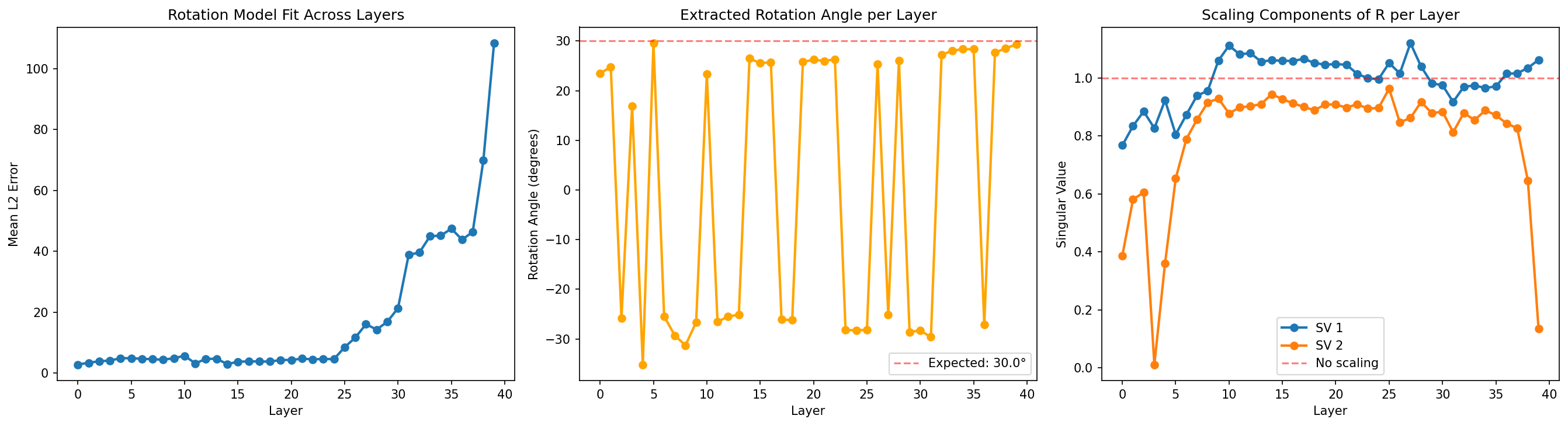
If the days formed a perfect circle, a single rotation matrix R should map each day's vector to its successor: R × Monday ≈ Tuesday, R × Tuesday ≈ Wednesday, etc. We fit such a matrix via least squares on the six consecutive pairs (Monday→Tuesday through Saturday→Sunday) in PCA space, then decompose it via Singular Value Decomposition (SVD) to understand its structure. SVD re-writes the matrix R as a set of three operations: a rotation, a stretch in each dimension (singular values), another rotation.

An additive "successor vector" — a single direction you add to any day to get the next — fundamentally cannot work on a circle, because the direction from Monday to Tuesday is roughly opposite to the direction from Thursday to Friday (it is not linear). The rotation matrix handles this by applying a different displacement depending on where the input vector is, rotating it around the circle.

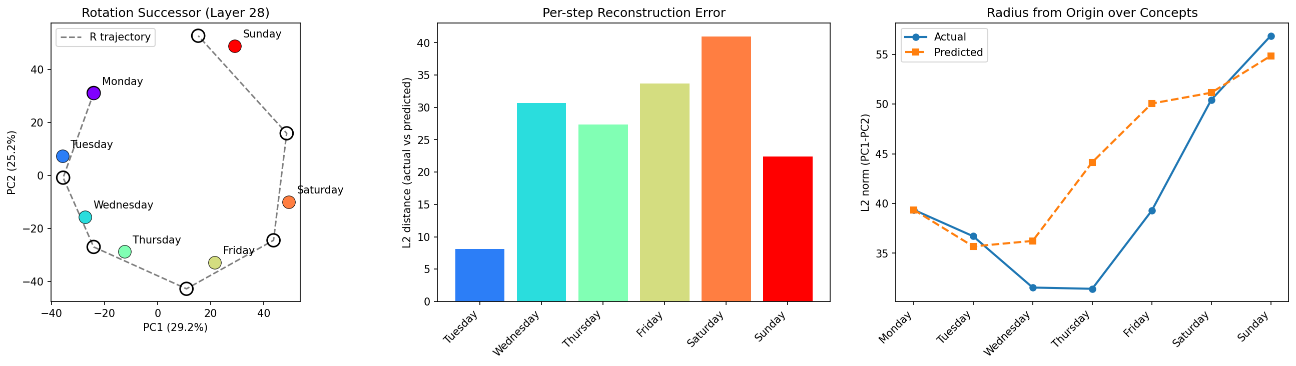
Starting from Monday and iteratively applying R six times traces a trajectory that sort of follows the actual day positions, with error accumulating primarily at the Sunday end. If we plot the radius of each day we see a general increasing trend, consistent with the spiral structure.

The Window of Circularity

The SVD decomposition of R reveals whether the successor operation is a pure rotation (singular values ≈ 1.0) or includes scaling (singular values ≠ 1.0). Tracking this across layers tells us where in the network the day-of-week representation is most circular.

We are most interested in what happens after layer ~6, as before this the model hasn't constructed a semantic representation of days at this stage. The first singular value (SV1) starts above 1.0 from about layer 10 to ~17 — indicating a circle with radial expansion. SV1 appears to drop toward 1.0 in a window around layers 17–30, reaching its minimum near layer 22. This is where the model's representation of days is most circular. On either side, the representation is more spiral-like. SV2 is consistently very close to one from layer 10 onwards , with a slight perturbation where SV1 goes through its turning point.

The extracted rotation angle stabilises near 51° (close to the ideal 360°/7 ≈ 51.4°) from around layer 10 onward, confirming that the model has built a coherent circular structure by the middle layers.

Months of the Year: Spiral, or Elliptical?

Repeating the analysis for the twelve months of the year produces a more elliptical shape. The December→January gap, while present, is smaller relative to other consecutive gaps than the Sunday→Monday gap is for days.

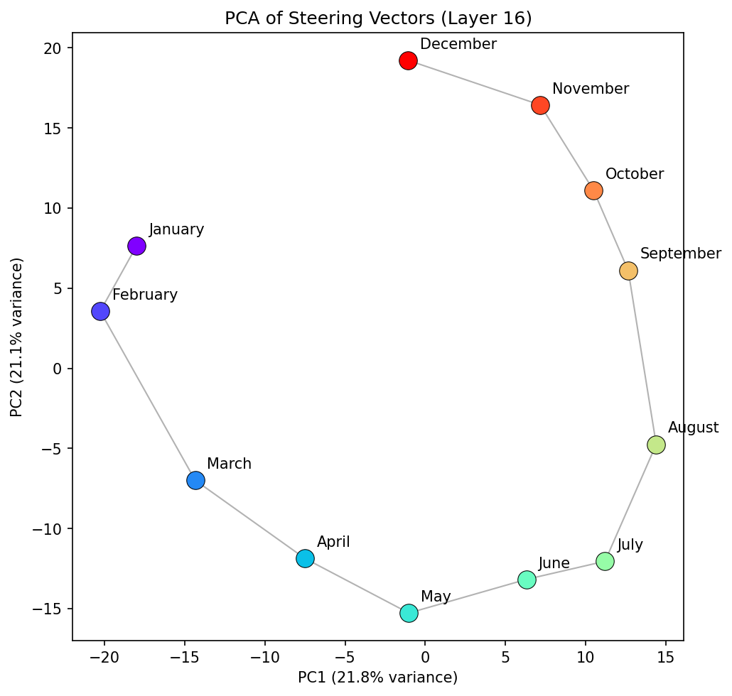
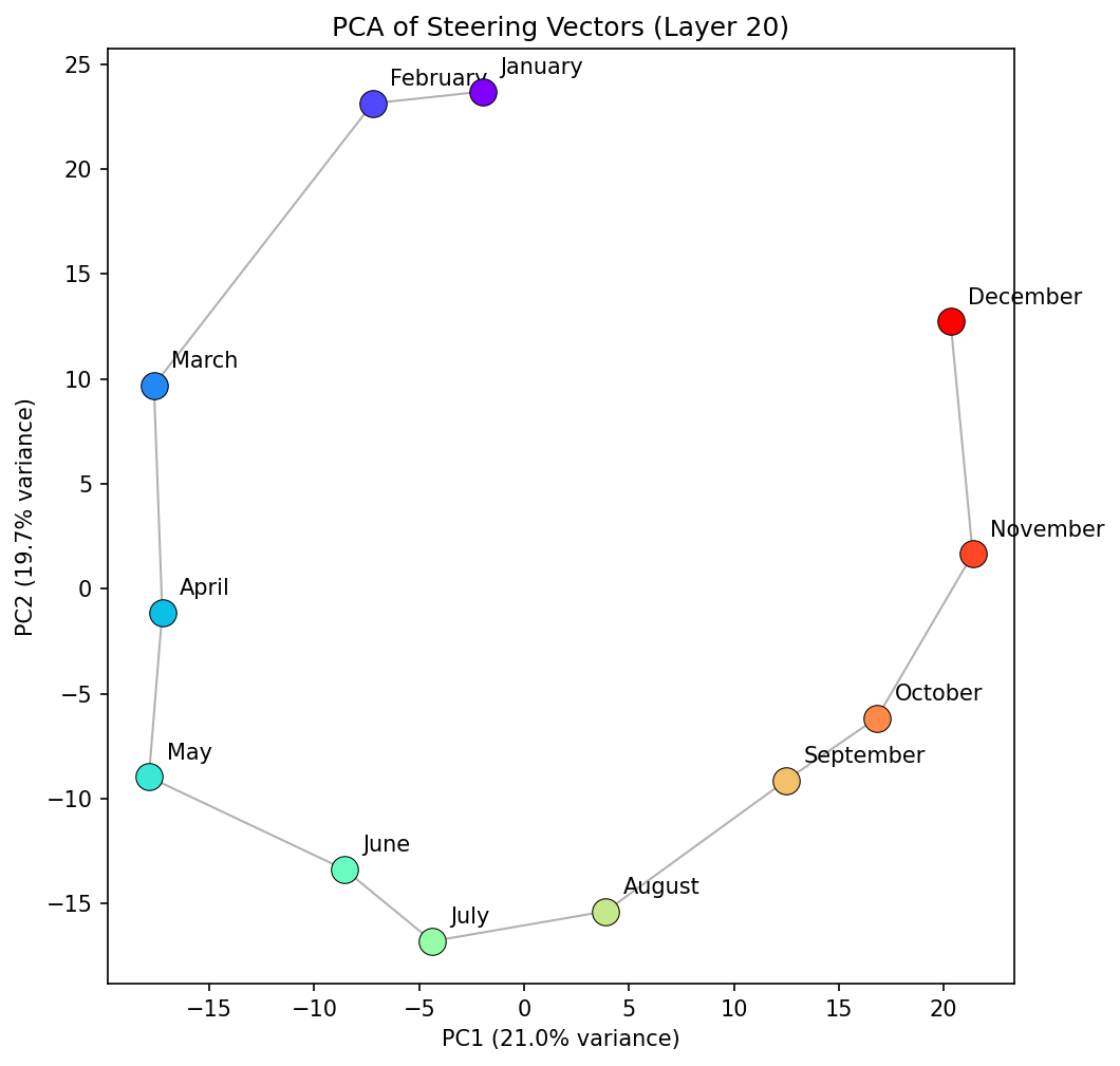
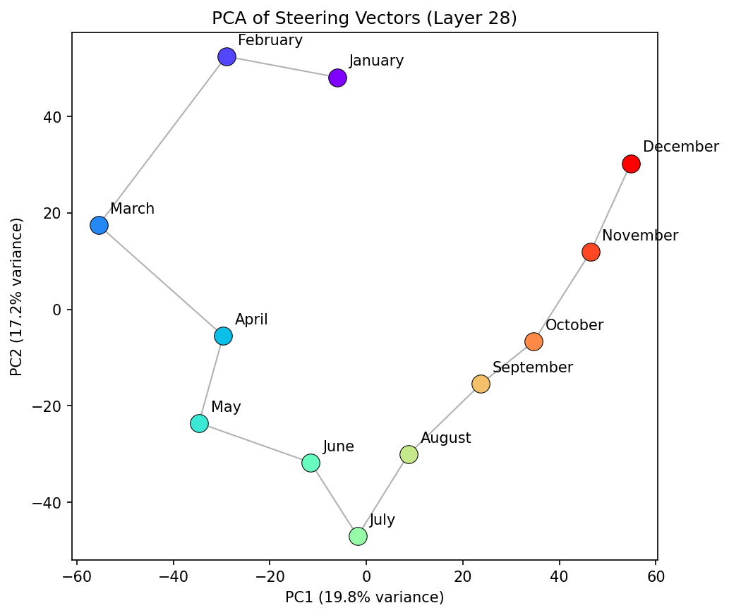
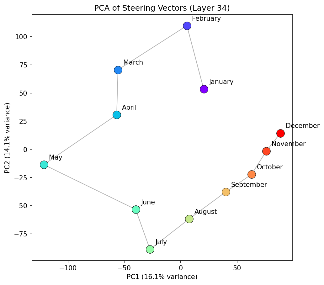
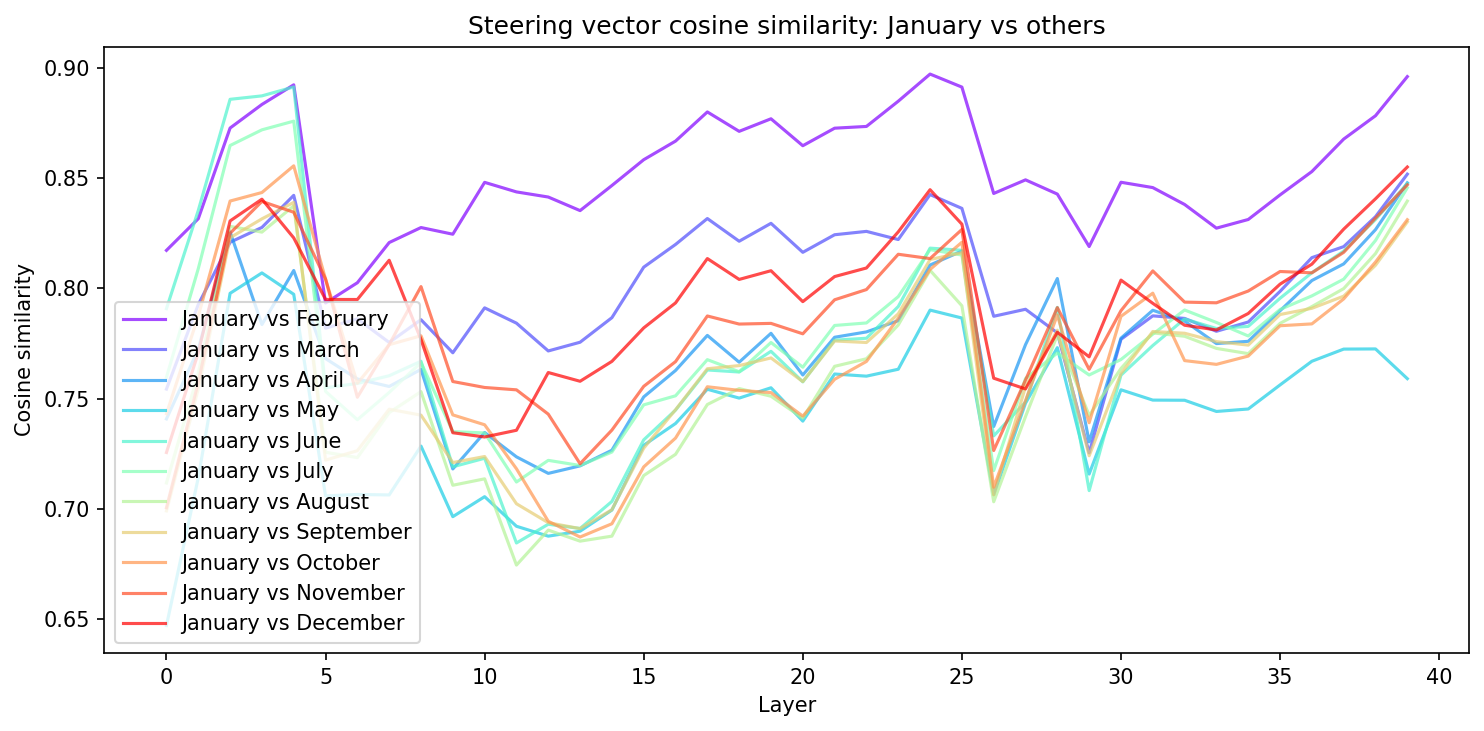
In the middle layers, the model seems to treat months as relatively periodic, similar to days, as we would expect. The PCA is more changeable than for the days concept family, however. The layer 20 PCA reflects elliptical structure, with a larger than average gap between January and December--consistent with the findings from the days of the week. It is also worth noting that neighbouring month distances seem to have more variance than in the days of the week case. For example, in layer 20 January and February are much closer than February and March. Does this arise because of a seasonal element? Is it because they end with "uary", or that the token "March" can have other semantic meanings and the model hasnt fully worked it through yet? At layer 25, the PCA space starts to break from a well described ellipse and forms a more complex structure. The representation during these layers (24 - 35) seem less stable than days of the week, and you likely lose information by projecting onto a 2D space. This notion is supported when we plot the cosine similarity between "January" and all other months. We see the coherent pattern between "January" and all other months becomes less defined after these middle layers.

The SVD of the months PCA space is only really valid on a 2D manifold in middle layers, before additional structure is added during later layers. The radial relationship between the months of the year are as expected, with "January" and "December" being maximum.

The elliptical notion becomes more obvious when we plot the singular values for the rotation matrix R as a function of layer. After layer 10, SV1 and SV2 seem to bridge unity from either side, suggesting our SVD squashes along one dimension and stretches along the other, a typical elliptical transformation. The angle between neighbouring concepts doesn't quite settle on the expected 30° (360°/12). One interesting point is that if the days of the week has some spiral structure, why are the months of year represented more elliptically? Is it that there exists semantic relationships that bridge the "January" -> "December" gap, e.g. Seasons, Public Holidays? The change from "Sunday" to "Monday" is more discontinuous, there is no real semantic tether between the concepts beyond neighbouring days of the week that I can think of.

Compass Directions: Geometry Across Layers

Compass directions provide a non-temporal test case. Using just the four cardinal directions (north, east, south, west), the results suggest the geometry changes qualitatively across layers.

At certain layers, the four directions form a clean square in PCA space, with PC1 corresponding roughly to the east-west axis and PC2 to north-south. This is consistent with spatial understanding — the representation encodes that north is opposite south, east is opposite west, and the two axes are perpendicular.

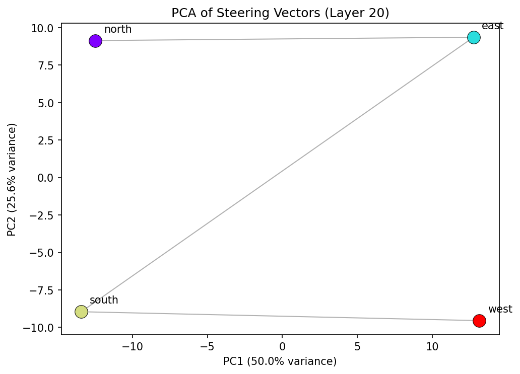
But at other layers, the square distorts into a trapezoid. North and south collapse together on PC2, while east and west remain separated. The cosine similarity between the north and south steering vectors is higher than between north and east — the model sees north and south as more similar to each other than either is to east or west.

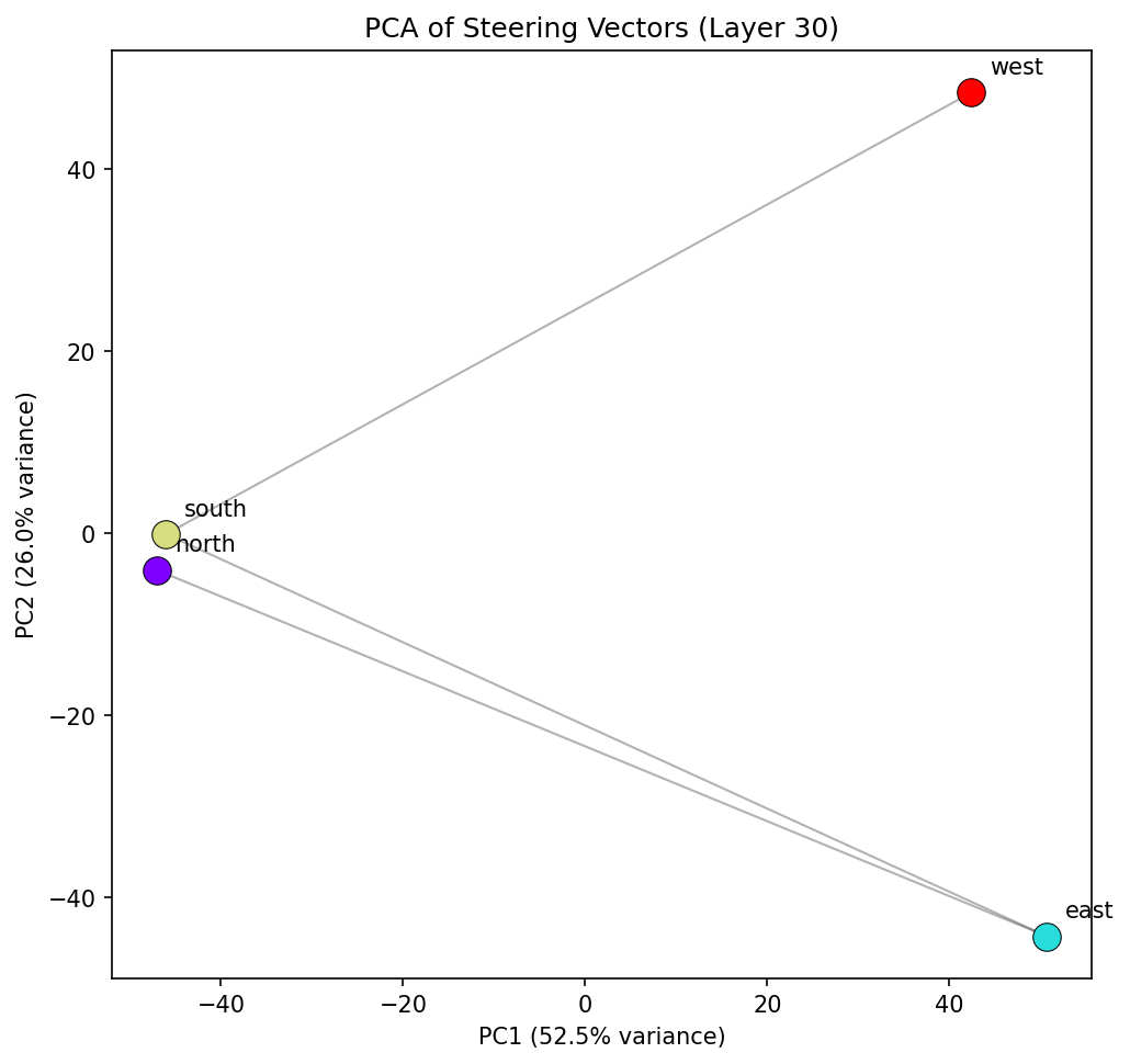
This likely is a feature of "north" and "south" having increased occurence together in natural language rather than spatial differences. "North" and "south" appear together in English: "north-south divide", "north to south", "northern and southern hemisphere", while "north" and "east" occur together less frequently. At these later layers, the model's representation is likely shaped more by how the words are likely to be used, as the concept family might fracture from purely spatial to more language influenced semantics.

Discussion

The main finding is that concept families occupy structured, low-dimensional subspaces in the residual stream at certain layers. It seems the geometry of these subspaces is also interpretable. The shape tells you something about how the model understands the concept family:

Periodicity vs linearity. Days form a spiral (mostly linear, partially periodic, throughout the entirety of the transformer). Months form an ellipse (in middle layers). This spectrum is quantifiable through the SVD of the fitted rotation matrix — singular values near 1.0 indicate pure rotation (periodicity), values above 1.0 indicate expansion (linearity).

Layer progression. The same concept family has different geometry at different layers. Early layers lack semantic structure. Middle layers encode the cleanest, most "faithful" geometric representation. Later layers distort the geometry as linguistic associations and task-specific features are mixed in. For compass directions, we see a potential transition from spatial understanding (square) to more linguistic understanding (trapezoid).

Boundary effects. Every concept family with an ordering shows some discontinuity (Sunday→Monday, December→January) but the magnitude varies and is smallest where the representation is most circular. These boundaries likely reflect the statistical structure of training data.

These are relatively simple analyses, but it suggests that looking at the geometry of concept families (and not just individual concept vectors) can reveal structure in how language models organise knowledge. The rotation analysis provides a simple quantitative framework for measuring how periodic a representation is, which could be applied to other concept families: musical keys, colour wheels, number systems, or any domain where concepts have relational structure.

All code and figures were produced using contrastive activation extraction on the Qwen3 13B parameter model, with thinking disabled. This model has separate Query heads for each of the 40 layers, however uses 8 Key and Value heads. The analysis requires only PCA, least-squares fitting, and SVD.

AI assistance

This work was heavily influenced by AI. In particular, Opus 4.5 wrote ~75% of the code for this project, and ~100% of the plotting code.

I also used Opus 4.5 to discuss some of the key findings in this work, in order to cement my understanding and ensure my discussion was more structured.